June 13, 2019
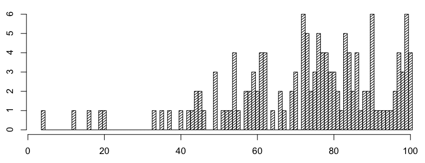
Here are some statistics from the 126 final (sections E and F only):
Min: 4; 1st Quartile: 60; Median: 76; 3rd Quartile 86; Max.: 100 (4 students (6 students had 99))
Here is a histogram of scores:
June 2, 2019
Here is a study guide for the final exam.
All problems on all old finals are worth studying, back at least a few years. I recommend starting with the more recent exams and working backward. Old final exams can be found on the 126 Materials Website (link at right).
June 1, 2019
Comments on actually using Taylor series to calculate trig functions. Suppose we wish to be able to calculate sin x for any x. The first thing we might notice is that sin is periodic with period 2 pi. This means that, for all x, there is a value x', such that sin(x)=sin(x') and x' is between -pi and pi. Further, because of the symmetry of the graph of sin, we can find a value x'' such that sin(x')=sin(x'') and x'' is between -pi/2 and pi/2. Further, we note that sin is an odd function, so sin(-y)=-sin(y). For these reasons, we need only worry about calculating sin x for x between 0 and pi/2.
Still further, we can note that cos(pi/2-x)=sin(x). This allows us to only deal with values between 0 and pi/4: if x is between pi/4 and pi/2, then pi/2-x is between 0 and pi/4.
So, what is needed are good ways to calculate sin x and cos x when x is between 0 and pi/4. Let's say we want 9 digits of accuracy (what your TI-30XIIS displays). An error of less than 10-10 would suffice. Let's shoot for 10-11 just to be on the safe side.
Then, by Taylor's inequality, and the fact that the all derivatives of sin x and cos x are bounded in absolute value by 1, we want to find n such that en=((pi/4)n+1)/((n+1)!)<10-11.
| n | en |
| 1 | 0.3084251375 |
| 2 | 0.08074551219 |
| 3 | 0.01585434424 |
| 4 | 0.002490394570 |
| 5 | 0.0003259918869 |
| 6 | 3.657620418 E-5 |
| 7 | 3.590860449 E-6 |
| 8 | 3.133616890 E-7 |
| 9 | 2.461136950 E-8 |
| 10 | 1.757247673 E-9 |
| 11 | 1.150115913 E-10 |
| 12 | 6.948453274 E-12 |
| 13 | 3.898073171 E-13 |
We see that n=12 will get us the accuracy needed.
That means that we can use the Taylor polynomialS(x)=x-x^3/6+x^5/120-x^7/5040+x^9/362880+x^11/39916800
to approximate sin x and the Taylor polynomial
C(x)=1-x^2/2+x^4/24-x^6/720+x^8/40320-x^10/3628800+x^12/479001600
to approximate cos x. Using these polynomials, we can approximate sin x for any x to a very good degree of precision. Using software with greater precision than the TI-30, we can do some calculations to verify how well these polynomials work.
The method then, to approximate sin x for x between 0 and pi/2, is to calculate as S(x) if x is less then pi/4, and as C(pi/2-x) if x is greater than pi/4.
Results are in the following table. Notice how many digits of agreement there are between sin x and the approximation. Note how the largest error (i.e., difference) occurs around pi/4, since that is the farthest away from the base (zero) that we have to deal with.
| x | approximation of sin x | sin x | difference |
| 0 | 0 | 0.E-19 | 0.E-19 |
| 0.10000000000000 | 0.099833416646828 | 0.099833416646828 | -2.0328790734103 E-20 |
| 0.20000000000000 | 0.19866933079506 | 0.19866933079506 | 1.2197274440462 E-19 |
| 0.30000000000000 | 0.29552020666134 | 0.29552020666134 | 2.5587171270658 E-17 |
| 0.40000000000000 | 0.38941834230865 | 0.38941834230865 | 1.0768838078212 E-15 |
| 0.50000000000000 | 0.47942553860418 | 0.47942553860420 | 1.9579986503676 E-14 |
| 0.60000000000000 | 0.56464247339483 | 0.56464247339504 | 2.0938318353453 E-13 |
| 0.70000000000000 | 0.64421768723614 | 0.64421768723769 | 1.5523208261349 E-12 |
| 0.80000000000000 | 0.71735609089982 | 0.71735609089952 | -2.9900057039664 E-13 |
| 0.90000000000000 | 0.78332690962753 | 0.78332690962748 | -4.2760879472720 E-14 |
| 1.0000000000000 | 0.84147098480790 | 0.84147098480790 | -4.4641482351004 E-15 |
| 1.1000000000000 | 0.89120736006144 | 0.89120736006144 | -3.0108294329922 E-16 |
| 1.2000000000000 | 0.93203908596723 | 0.93203908596723 | -1.0625181290358 E-17 |
| 1.3000000000000 | 0.96355818541719 | 0.96355818541719 | -1.0842021724855 E-19 |
| 1.4000000000000 | 0.98544972998846 | 0.98544972998846 | 1.5041360233406 E-22 |
| 1.5000000000000 | 0.99749498660405 | 0.99749498660405 | -4.2628003683383 E-23 |
And this is, essentially, what a calculator does: it creates an approximation to sin x that is so close to sin x that there is no point in being more accurate: a more accurate approximation would still be displayed as the same number.
In practice, calculators usually calculate to a higher degree of precision than is implied by their displayed digits, in order to reduce error during computations, but the method is similar.
June 1, 2019
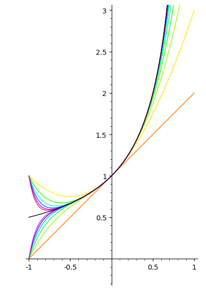
Here is a plot of y=1/(1-x) (in black) along with its first 12 Taylor polynomials. The higher degree ones are farther along the spectrum toward violet. We can see that the higher the degree, the close the polynomial agrees with 1/(1-x). There is a simple relationship on the right of the y-axis, but on the left, the polynomials behave one of two ways depending on the degree: if the degree is even, then the the curve bends upward away from y=1/(1-x), and if the degree is odd, then the curve must pass through (-1,0), and so they bend downward away from y=1/(1-x).
May 29, 2019
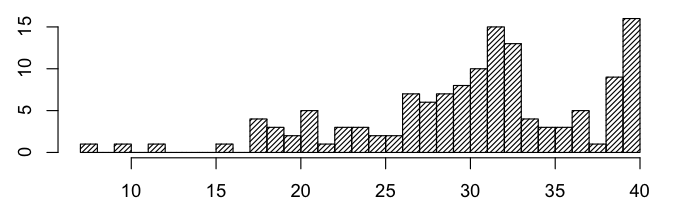
Midterm Two statistics: min=7; 1st quartile =27; median=32; 3rd quartile=35.25; max=40 (16 students)
Here is a histogram of exam scores from Midterm Two:
Answers to the second midterm exam are in the exam archive.
May 20, 2019
Here is a basic skills list for Midterm Two.
May 17, 2019
I added an example of a volume calculation involving a quadric surface to the resources in the right-hand column.
Here are some problems from old exams that are worth studying for the upcoming second midterm exam.
- Spring 2012, MT2, #1, 2, 4, 5
- Spring 2011, MT2, all problems
- Autumn 2010, MT2, #1, 2, 3, 5
- Spring 2010, MT2, #3, 4
- Spring 2009, MT2, #3, 4, 5
- Spring 2008, MT2, #5
- Spring 2007, MT2, #5
May 7, 2019
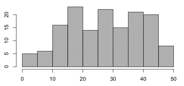
Midterm One statistics: min=0; 1st quartile=18.25; median=27.5; 3rd quartile=38.0; max=50 (1 student)
Here is a histogram of exam scores from Midterm One:
Grade interpretation: assuming a median course grade of 2.7 (the minimum it could be, so this gives a lower bound), you can approximate your 4.0-scale grade interpretation of your Midterm One exam score as follows:
- If your score was 46 or above, your grade interpretation is approximately 4.0.
- If your score was between 28 and 46, your interpretated grade is approximately 2.7+0.072(score-28).
- If your score was between 20 and 28, your interpreated grade is approximately 2.7+0.2(score-28).
- If your score was less than 19, your interpretated grade is approximately 0.0.
Answers to midterm one are now in the exam archive (link at right).
May 1, 2019
Regarding Spring 2010, MT1, #4. In this problem, students were
asked to find the equation of the surface that is the set of points
which are twice as far from the z-axis as from the x-axis. As we discussed,
the distance from a point (x,y,z) to the z-axis is (x2+y2)1/2
and the distance from (x,y,z) to the x-axis is (y2+z2)1/2.
The surface we are interested in consists of points for which the first distance is
twice the second: they must satisfy the equation
(x2+y2)1/2 = 2 (y2+z2)1/2.
The square roots don't help us, so we get rid of them:
x2+y2 = 4 ( y2+z2 )
and finally
x2 -3 y 2 -4z2= 0.
This equation is quadratic in all three variables, and defines a quadric surface.
If x is replaced by a constant, then the equation defines an ellipse.
If y is replaced by a constant, then the equation defines a hyperbola.
If z is replaced by a constant, then the equation defines a hyperbola.
Since two traces are hyperbolas, the surface is a hyperboloid.
I like to call it an elliptic hyperboloid, but this is actually redundant: if two
traces are hyperbolas, then the other must be an ellipse (why?).
People just call these sorts of surfaces hyperboloids.
We saw previously that there are three types of hyperboloids: hyperboloids of one sheet,
cones, and hyperboloids of two sheets.
If we have a standard form equation of our quadric surface, and we do, then a quick
way to tell that it is a cone is to notice that it passes through the origin: hyperboloids
of one or two sheets (in standard form) will not pass through the origin.
We can also note that our equation can be written as 3y2+4z2=x2.
So, if we set x to a constant, then we get ellipses (as we saw when we considered traces).
This means that if we slice through the surface at the plane x=c, then we get an ellipse.
In the case when x=0, we get what is called a degenerate ellipse: it is simply the point (0,0,0).
As we move away from x=0 in the positive x direction, the ellipse gets larger and larger.
Further, we can note that the "size" of the ellipse is a linear function of x=c.
For example, with x=c, setting z=0 gives us y2 = (1/3)c2, so y=± c/3.
That is, the "width" in the y dimension is 2c/3, and so the width increases linearly with c.
The same is true for the "width" in the z dimension.
This linearity in the size of the elliptical cross section as a function of x exactly characterizes cones, and only
cones, among the quadric surfaces.
Getting still more elaborate, if you slice through the surface with a plane that contains the x-axis
and makes an angle of θ with the xy-plane, the intersection is a pair of lines parametrizable as
x=t, y = ± t/(3+4 tan2 θ)1/2, y = ± (t tan θ)/(3+4 tan2 θ)1/2 .
This linearity again is characteristic of the cone.
Finally, if you look at the table given in class, we see the standard form with all variables
quadratic and the right-hand size equal to zero is classified as a cone: that's a nice, easy
way to tell that this surface is a cone.
April 26, 2019
Here are some suggested problems in my exam archive (link at right) that are worth working in preparation for the first midterm exam. I recommend starting with the exams for which all problems are relevant, and then move on to the other ones.
- Spring 2012, MT 1: all problems
- Spring 2011, MT 1: all problems
- Autumn 2010, MT 1: 1-4, 5(a)
- Spring 2010, MT 1: all problems
- Spring 2010, MT 2: 1, 2
- Spring 2009, MT 1: 1,2,4,5
- Spring 2009, MT 2: 1, 2
- Spring 2007, MT 1: 3, 4, 5
- Spring 2007, MT 2: 1, 2, 3, 4
- Spring 2006, MT 1: 3, 4, 5, 6
- Spring 2006, MT 2: 2, 3, 3, 5
Here is a study guide for the first midterm exam.
Some comments on today's lecture. Curvature is a critical concept in train track design. To transition from one piece of track to another, it is critical that the curvatures are equal at the point of transition. In order to transition from a curved track to a straight track (which has zero curvature), the curvature of the curved track must decrease to zero at the point of transition. The curvatures must be equal at the point of transition in order to avoid having a sudden change in acceleration (mathematically, an unbounded third derivative), which, at best, would be felt as a sudden jerk, and at worst, would derail the train.
As we saw in class, the curvature of y=x2 decreases to a minimum of 2 as x approaches zero from the left. As a result, if we tried to make a track transition from the curve y=x2 to the straight, positive x-axis at the origin this would result in an instantaneous change in curvature (from 2 to 0) as the train passed the origin.
If we consider the same scenario with the curve y=x4, we see that a smooth transition is possible since the curvature of y=x4 decreases to zero as x approaches zero from the left. Since the positive x-axis also has curvature zero, a train transitioning from y=x4 to the positive x-axis would not experience an instantaneous change of curvature.
A specialized curve known as Cornu's spiral is commonly for designing transitions between pieces of train track or sections of roadway. A useful feature of this spiral is it that it contains points of all possible curvatures.
April 22, 2019
More comments on today's lecture. Today we discussed the polar curve r = cos θ. We saw that the curve is a circle (with center (1/2, 0) and radius 1/2). The curious thing about this polar curve is that the curve is traversed twice as θ runs from 0 to 2π.
Here we have the graph of y = cos x, to show the relationship
between r and θ that we get from the equation r = cos θ:
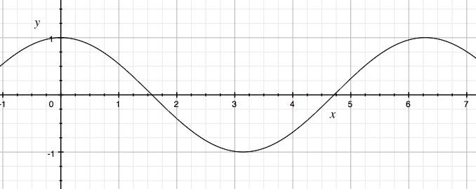
As θ runs from 0 to π, we see r changes from 1 to -1.
As we discussed in class, this gives us the entire curve.
(Note that the polar point (-1, π) is the cartesian point (1,0), the
same point as the polar point (1,0).)
Then as we continue letting θ run from π to 2π, the
radius goes from -1 to 1, and we find that this gives us another tracing
of the curve.
At that point, because cos θ is periodic with period 2 π,
if we continue letting θ increase beyond 2 π we retrace
the curve over and over.
For practice, try drawing the curve given by r= cos2 θ.
You'll see that this curve is only traversed once as θ goes from
0 to 2π.
Lines. In class, we saw that the line y=mx+b has polar equation
r = b/(sin θ-m cos θ).
A sharp student pointed out that, since we have a division happening,
there is a danger that we might divide by zero. At the same time, we
can notice that, if b=0, then this equation is nonsense: we just get r=0
which is clearly not the polar equation for a line.
What gives?
Note that, if b=0, then the line passes through the origin.
In that case, y = mx for any point (x,y) on the line, and so
the polar representation of this point satisfies r sin θ = m cos θ,
and so sin θ - m cos θ = 0.
So, for lines with b=0, this polar equation is nonsense; instead,
we can specify the line by the simple equation θ=atan(m).
Further, note that sin θ-m cos θ=0 only if b=0, since
sin θ - m cos θ=0 implies y-mx=0.
So, we have r = b/(sin θ-m cos θ) for lines with b not equal to zero,
and θ=atan(m) for line with b=0.
Notice that this is analogous to the situation with cartesian equations of lines:
if a line if not vertical, we can express it as y=mx+b, and if it is vertical,
then it can be expressed as x=c for some constant c.
April 19, 2019
More on the "pitch" of a circular helix
In class, we saw that the helix r(t) = < cos t, sin t, t > makes
an angle of 45 degree with any plane parallel to the xy-plane.
What about the helix r(t) = < cos t, sin t, at >, for any real positive a?
The derivative is r'(t) = <-sin t, cos t, a> and
so the dot product of r'(t) with the plane's normal vector <0,0,1> is a.
Since |r'(t)| = sqrt(1 + a2), we are able to conclude that
the angle θ between r'(t) and the normal vector satisfies
cos θ = a/sqrt(1+a2).
Given a value of a, from this we can calculate θ.
Suppose we want the angle to be 22 degrees. What should a be?
Since we want an angle of 22 degrees between the curve and the plane,
we need an angle of 90-22=68 degrees between r'(t) and <0,0,1>.
That is, we want θ=68 degrees = 1.186823... .
To find the right value of a, we use the fact that
cos 1.186823... = 0.3746.. = a/sqrt(1 + a2).
Solving, we find a = 0.404026... .
With a=1, we got 45 degrees. As we'd expect, the get a lower angle (22 versus 45), the helix needs to "rise" at a slower rate, and this smaller value of a achieves that.
April 17, 2019
A quick comment about the conical helix. Today we talked briefly
about the parametric curve x=t cos t, y=t sin t, z=t, and we concluded
that it was similar to a helix with increasing "radius" the farther
it got from the origin. I said it was called a "conical helix".
We can quickly see why: for any t, we can note
that
(t cos t)2+(t sin t)2-t2
= t2 (cos2 t +sin2 t) - t 2
= t2 - t2 = 0.
Hence, every point on our curve satisfies the equation
x2+y2-z2=0.
We saw on Monday that this is the equation of a surface called a cone
(notice that, if we slice through this surface at z=k, we get a circle of radius |k|:
a point at the origin, and increasingly large circles as we move away from the xy-plane.)
Thus, the curve lies on a cone, and that's why we call it a conical helix.
April 17, 2019
CLUE will be holding reviews for exams at these times:
- Midterm 1 Review: Tuesday, April 23rd (8-9:30pm)
- Priority Drop-in Midterm 1: Tuesday, April 30th (7-9pm)
- Midterm 2 Review: Monday, May 20th (6:30-8pm)
- Final Review: Friday, June 7th (7-9pm)
March 28, 2019
Welcome to Math 126E,F !
Announcements and other important information will appear here, so check back frequently.
The homework for this course will be on WebAssign.
Information on purchasing access to, and logging into WebAssign is here.
The first homework assignment will be due by 11 PM on April 9.
The course discussion board is now availble (link at right). Please take advantage of it to ask questions about homework problems or course topics. You might also use it as a way to arrange study groups. I will get immediate emails when posts are added to the board, so this is as good a way to contact me as email, but allows everyone to see my response.
In case you would like to "look ahead" in the course, here is a rough calendar for topics we will be covering. It is subject to change.
| Week 1 | 3D coordinate system, vectors, dot product | 12.1,12.2,12.3 |
| Week 2 | cross product, lines and planes in 3D | 12.4, 12.5 |
| Week 3 | cylinders and quadric surfaces, vector functions and space curves, calculus on vector functions | 12.6, 13.1, 13.2 |
| Week 4 | polar coordinates, arc length, curvature, velocity and acceleration | 10.3, 13.3, 13.4 |
| Week 5 | midterm one, functions of several variables | 14.1 |
| Week 6 | partial derivatives, tangent planes and linear approximations, max and min values | 14.3, 14.4, 14.7 |
| Week 7 | double integrals | 15.1, 15.2, 15.3 |
| Week 8 | applications of double integrals, midterm two, Taylor polynomials | 15.4, Taylor notes |
| Week 9 | Taylor series | Taylor notes |
| Week 10 | Taylor series | Taylor notes |