Some of the main results of Chapters 3 and 4

Chapter 3.

Let's start with the notion of a field. When you row reduce a matrix, or invert a matrix, or solve a system of linear equations, you need to perform the following operations: addition, subtraction, multiplication, and division. A field is defined precisely to make this possible, so a field is a set F with two operations, addition and multiplication, satisfying various properties (addition makes Finto an abelian group with identity element 0, multiplication makes $F^{\times} = F-\{0\}$ into an abelian group with identity element 1, and addition and multiplication are related to each other by the distributive law). You know several examples: the real numbers R, the complex numbers C, and the rational numbers Q. Another important example is the set of congruence classes of integers modulo a prime number p, written as Z/ p Z, or to emphasize that it's a field, as F_p.

Given a field F (and if you want, just take F=R or F=C), a vector space over F is a set V together with two operations: addition (also known as ``vector addition''; this makes V into an abelian group), and scalar multiplication. These have to satisfy the axioms listed in Definition 2.11. (See also Definition 1.6 for the special case when F= R.) Standard example: Rⁿ, the length n column vectors with real entries, is a vector space over R. (More generally, for any field F, Fⁿ is a vector space over F.) Any line through the origin or plane through the origin in R³ is a vector space, and is a subspace of R³. The complex plane C can be viewed as a vector space over C, over R, or over Q, just by restricting which sorts of numbers you allow for scalar multiplication.

Now fix a field F and a vector space V over F. The elements of V are called vectors, of course, and the elements of F are called scalars. If v₁, ..., v_n are vectors in V, then a linear combination of these vectors is any vector of the form

$$a_{1} v_{1} + \dotsb + a_{n} v_{n},$$

where a₁, ..., a_n are scalars. The set of all linear combinations of the vectors v₁, ..., v_n is the subspace spanned by the set, written

$$\Span (v_{1}, \dotsc, v_{n}).$$

It is a subspace of V. For example,

$$\Span (\begin{bmatrix} 1 & 0 & 0 \end{bmatrix}^{t}, \begin{bmatrix}0 & 1 & 0 \end{bmatrix}^{t})$$

is the (x,y)-plane in R³, as is

$$\Span (\begin{bmatrix}1 & 0 & 0 \end{bmatrix}^{t}, \begin{bma... ...end{bmatrix}^{t}, \begin{bmatrix}2 & 3 & 0 \end{bmatrix}^{t}).$$

A set of vectors v₁, ..., v_n is linearly dependent if

$$a_{1} v_{1} + \dotsb + a_{n} v_{n} = 0$$

for some scalars a₁, ..., a_n which are not all zero. Otherwise, the set is linearly independent. For example, the set

$$\begin{bmatrix}1 & 0 & 0 \end{bmatrix}^{t}, \begin{bmatrix}0 ... ... \end{bmatrix}^{t}, \begin{bmatrix}2 & 3 & 0 \end{bmatrix}^{t}$$

is linearly dependent, because

$$2\begin{bmatrix}1 & 0 & 0 \end{bmatrix}^{t} + 3 \begin{bmatri... ...bmatrix}^{t} - \begin{bmatrix}2 & 3 & 0 \end{bmatrix}^{t} = 0.$$

The set

$$\begin{bmatrix}1 & 0 & 0 \end{bmatrix}^{t}, \begin{bmatrix}0 & 1 & 0 \end{bmatrix}^{t}$$

is linearly independent.

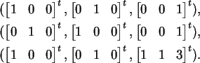
A basis for a vector space V is a set of linearly independent vectors in V which also spans V. For some computations, it is useful to pay attention to the order of elements in a basis, so a basis is actually an ordered set of linearly independent vectors which span the space. For example, the following are (different) bases for R³:
$$\begin{gather*}(\begin{bmatrix}1 & 0 & 0 \end{bmatrix}^{t}, \begin{bmatrix}0 &... ... \end{bmatrix}^{t}, \begin{bmatrix}1 & 1 & 3 \end{bmatrix}^{t}). \end{gather*}$$
(Standard notation: if you list elements in curly braces - $\{x,y\}$- that means a set. If you list them in parentheses - (x,y) - that means an ordered set. So the sets $\{x,y\}$ and $\{y,x\}$ are equal, while the ordered sets (x,y) and (y,x) are different.)

Proposition 3.8 is important: a set $\mathbf{B} = (v_{1}, \dotsc, v_{n})$ is a basis if and only if every vector $v \in W$ can be written as a linear combination of the v_i's, in a unique way.

On to a discussion of dimension: first, a vector space V is finite-dimensional if there is a finite set of vectors which spans it. (E.g., I gave several different finite sets which span R³.) Assume that V is finite-dimensional; then Proposition 3.17 says that any two bases for V have the same number of elements, so define the dimension of V to be the number of vectors in any basis. (E.g., the dimension of R³ is 3.)

Given a vector space V and a basis $\mathbf{B} = (v_{1}, \dotsc, v_{n})$, any vector $v \in V$ can be written in exactly one way as a linear combination

$$v = a_{1} v_{1} + \dotsb + a_{n} v_{n}.$$

The coefficients $(a_{1}, \dotsc, a_{n})$ are called the coordinates of v with respect to the basis B. (This is the first place where the order of the basis vectors is important: if I permute the elements of the basis around, that will also permute the coordinates of v.)

Suppose we are working with the vector space Rⁿ of n-dimensional column vectors with real entries. The standard basis for Rⁿ is

$$\mathbf{E} = (e_{1}, e_{2}, \dotsc, e_{n}),$$

where e_j is the column vector with 1 in the jth spot and 0's elsewhere. If I have some other basis $\mathbf{B} = (v_{1}, \dotsc, v_{n})$ for Rⁿ (see above for some examples with R³), and if I have a vector $Y = \begin{bmatrix}y_{1} & \dotsb & y_{n} \end{bmatrix}^{t}$ in Rⁿ, then Proposition 4.7 tells me how to compute the coordinates of Y with respect to the basis B: form a matrix [B] in which the jth column is the vector v_j. Then the coordinates of Y are given by [B]^-1 Y. (So if X = [B]^-1 Y, then $Y = x_{1} v_{1} + x_{2} v_{2} + \dotsb + x_{n} v_{n}$.)

More generally, given two different bases for a vector space V, it is important to be able to convert between one and the other. See pages 97-99 for a discussion of this.

(I'm not going to discuss the material in Sections 3.5 and 3.6 now, but I'll ask you to read them eventually.)

Chapter 4.

Given two vector spaces V and W over a field F, a linear transformation from V to W is a function

$$T : V \longrightarrow W$$

which satisfies two properties: T(v + v') = T(v) + T(v') for any two vectors $v, v' \in V$, and T(av) = a T(v) for any $a \in F$ and $v \in V$. For example, left multiplication by an $m \times n$ matrix defines a linear transformation from Rⁿ to R^m.

Notice that if we ignore scalar multiplication, then any linear transformation T is a group homomorphism, so we can define the kernel and image of T. The kernel is also called the null space. One important formula is given in Theorem 1.6: for any linear transformation $T : V \longrightarrow W$,

$$\dim V = \dim (\ker T) + \dim (\im T).$$

By the way, the dimension of the kernel of T is also called the nullity of T, and the dimension of the image is also called the rank.

As it stands, linear transformations are somewhat abstract, while matrix multiplication is much more concrete. We can remedy this (and I don't mean by making matrix multiplication more abstract). First we have to choose a basis $\mathbf{B} = (v_{1}, \dotsc, v_{n})$ of Vand a basis $\mathbf{C} = (w_{1}, \dotsc, w_{m})$ of W. Then for each j, T(v_j) is in W, so can be written uniquely as a linear combination of the elements of C:

$$T(v_{j}) = a_{1j} w_{1} + a_{2j} w_{2} + \dotsb + a_{mj} w_{m},$$

for some scalars a_1j, ..., a_mj. So we can define an $m \times n$ matrix A with these scalars as entries. This is the matrix associated to the linear transformation T, with respect to the bases B and C. Now if v is a vector in V with coordinates $X = \begin{bmatrix} x_{1} & \dotsb & x_{n} \end{bmatrix}^{t}$, by which I mean that

$$v = x_{1} v_{1} + \dotsb + x_{n} v_{n},$$

then to compute T(v), you multiply the $m \times n$ matrix A by the $n \times 1$ matrix X to get an $m \times 1$ matrix Y; this matrix Y gives the coordinates of T(v) with respect to the basis C.

Here's a good example to work out: let P_n be the vector space of all real polynomials of degree at most n, with basis $(1, x, x^{2}, \dotsc, x^{n})$. Then the derivative D is a linear transformation from P_n to itself. Find the matrix for D with respect to this basis.

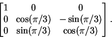
Another example of a linear transformation: let T be rotation of R³ by angle $\pi/3$ around the line through the origin determined by the vector $v = \begin{bmatrix}1 & 1 & 2 \end{bmatrix}^{t}$. I could work out the matrix for this with respect to the standard basis, but things will be nicer if I use v as, say, the first element of the basis. Since the linear transformation sends v to itself, then the matrix will look like

$$\begin{bmatrix} 1 & * & * \\ 0 & * & * \\ 0 & * & * \end{bmatrix},$$

where the *'s depend on how I choose the other two elements of the basis. If I choose the rest of the basis well, I'll end up with this for the matrix:

$$\begin{bmatrix} 1 & 0 & 0 \\ 0 & \cos(\pi/3) & -\sin(\pi/3) \\ 0 & \sin(\pi/3) & \cos(\pi/3) \end{bmatrix}.$$

If I'm willing to choose different bases for the domain and range of the function, then I can actually get the matrix to look like this:

$$\begin{bmatrix} 1 & 0 & 0 \\ 0 & 1 & 0 \\ 0 & 0 & 1 \end{bmatrix}.$$

How? Pick any basis B=(v₁, v₂, v₃) for R³(the domain); then the rotated vectors T(v₁), T(v₂), T(v₃) form a basis for R³, and I'll use this basis for the range. You get the identity matrix when you compute relative to these two bases.

If you change bases in either V or W or both, you get a new matrix for the linear transformation T; how a matrix is transformed when you change bases is discussed on pages 113-115. See Proposition 2.9, in particular.

If V is a vector space, then a linear operator on V is a linear transformation from V to itself. In this case, when computing a matrix for V, you usually pick the same basis for V in its role as domain and in its role as range. Proposition 3.5 says this: if A is the matrix for T with respect to some basis, then when you change bases, you get matrices of this form: PAP^-1, where P is in GL_n(F). Definition: two matrices A and A'are similar if A' = PAP^-1 for some invertible P.

Invariant subspaces, eigenvalues, and eigenvectors are used to study linear operators on a vector space V. A subspace W of V is invariant under T if $T(w) \in W$ for all $w \in W$. For example, if $T : \mathbf{R}^{3} \longrightarrow \mathbf{R}^{3}$ is rotation about the z-axis by angle $\pi/5$, then the xy-plane is an invariant subspace: given any vector v in the xy-plane, then T(v) is also in the xy-plane. The z-axis is another invariant subspace.

An eigenvector for T is a nonzero vector v so that Tv is a scalar multiple of v: Tv = cv for some $c \in F$. The scalar c is the eigenvalue associated to the eigenvector v. Corollaries 3.10, 3.11, and 3.12 are all important.

To find eigenvectors and eigenvalues, rewrite the equation Tv = cvas Tv = cIv, where I is the $n \times n$ identity matrix, and then rewrite this as cIv - Tv = 0, or (cI-T)v = 0. So a nonzero vector v is an eigenvector of T, with eigenvalue c, if v is in the kernel of cI-T. A matrix (or linear operator) has nonzero vectors in its kernel if and only if its determinant is zero, in which case it's called singular. So c is an eigenvalue for T if and only if the linear operator cI-T is singular, which is true if and only if $\det (cI-T) = 0$.

So, let T be a linear operator with matrix A, let t be a variable, and define the characteristic polynomial of T to be $p(t) = \det (tI - A)$. The eigenvalues of T are the roots of this degree n polynomial.

(This means that they are the roots of the polynomial that exist in the field F. So if we decide to work with the field Q of rational numbers, then the matrix $\begin{bmatrix}0 & 2 \\ 1 & 0 \end{bmatrix}$, which has characteristic polynomial p(t) = t² - 2, has no eigenvalues. It has two eigenvalues, $\sqrt{2}$ and $-\sqrt{2}$, if we are working over the field R.)

Corollary 4.14 and Proposition 4.18 are useful.

If T is a linear operator on a vector space V, it is useful to know whether T is similar to an upper triangular matrix or to a diagonal matrix. The characteristic polynomial is important here; see Corollary 6.2 and Theorem 6.4 for the main results.

Go to the Math 403 home page.

Go to John Palmieri's home page.