Take the four points in 3D space: (0,0,0),(1,0,0),(1,1,0),(0.5,0.5,1).
Calculate the distances between all pairs.
Enter in R:
> D <- matrix(c(0.0,1.0,1.4142135623730951,1.224744871391589,1.0,0.0,1.0,1.224744871391589,1.4142135623730951,
1.0,0.0,1.224744871391589,1.224744871391589,1.224744871391589,1.224744871391589,0.0),nrow=4,ncol=4,byrow=TRUE)
> D
         [,1]     [,2]     [,3]     [,4]
[1,] 0.000000 1.000000 1.414214 1.224745
[2,] 1.000000 0.000000 1.000000 1.224745
[3,] 1.414214 1.000000 0.000000 1.224745
[4,] 1.224745 1.224745 1.224745 0.000000
Use the cmdscale function to get a 1-dimensional model:
> cmdscale(D,k=1,eig=TRUE)
$points
              [,1]
[1,]  7.071068e-01
[2,]  4.440892e-16
[3,] -7.071068e-01
[4,] -8.326673e-17

$eig
[1] 1.000000e+00 8.201941e-01 3.048059e-01 6.661338e-16

$x
NULL

$ac
[1] 0

$GOF
[1] 0.4705882 0.4705882
From the $points section, we see the model has places two points essentially at the origin, and then two symmetrically at about 0.7 and -0.7.
We see from the eigenvalues that the first three are much, much larger than the fourth one. This suggests that a 3-dimensional model will work well.
Note that all eigenvalues here are positive. This will not be true in all cases. Negative eigenvalues indicate that the distances are non-euclidean, which means that no euclidean model will fit perfectly.
The goodness of fit is report here as 0.4705882 with both calculation methods. Enter
> ?cmdscale
to read about the two methods R uses to calculate goodness of fit. Note that the two values will be identical when all the eigenvalues are positive.
We can plot the model in 1D. It is something else.
> model1 <- cmdscale(D,k=1)
> for1Dplot <- data.frame(model1,0)
> plot(for1Dplot)
> mylabels <- c(1,2,3,4)
> text(for1Dplot,labels=mylabels,pos=4)
This gives us this plot:
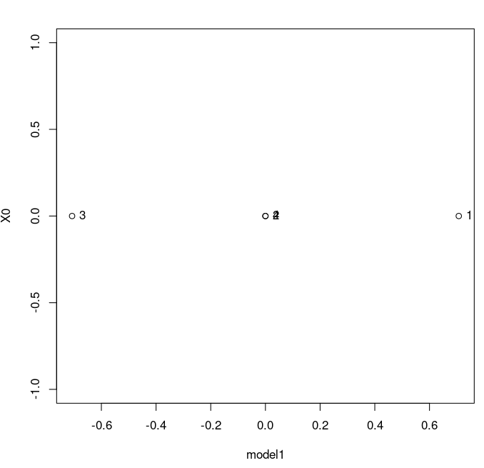
The label for 0 and 4 are overlapping, which we could fix, but let's not worry about it now. Warning: note that if you simply say plot(model1), you will get a plot where the x-axis is simply the index of the values, and the y-axis is the coordinate of your model. This is not what you want. It looks like this:
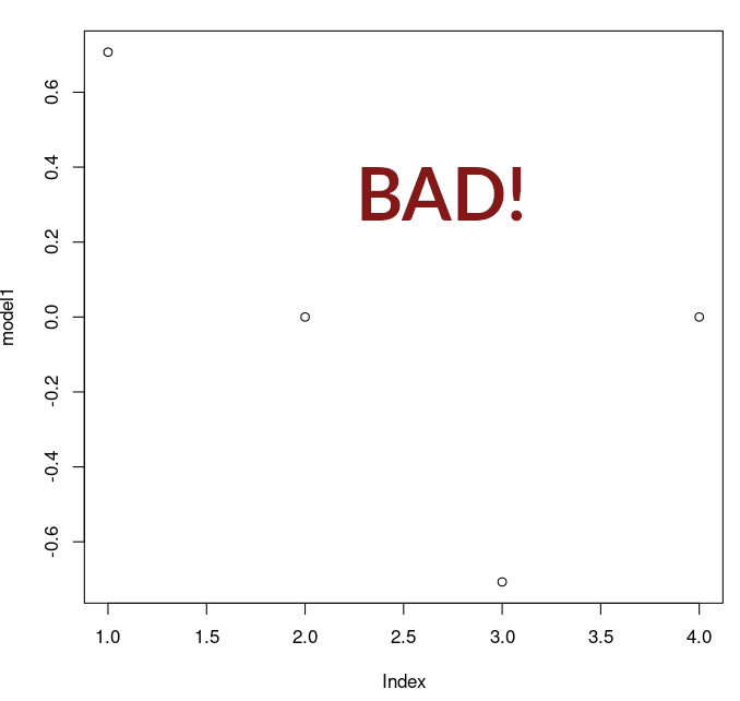
We can see that this is not a picture of the 1D model.
Moving on to a 2D model:
    > model2 <- cmdscale(D,k=2,eig=TRUE)
> model2
$points
              [,1]       [,2]
[1,]  7.071068e-01 -0.1671134
[2,]  4.440892e-16 -0.4280699
[3,] -7.071068e-01 -0.1671134
[4,] -8.326673e-17  0.7622968

$eig
[1] 1.000000e+00 8.201941e-01 3.048059e-01 6.661338e-16

$x
NULL

$ac
[1] 0

$GOF
[1] 0.8565619 0.8565619
We see the first-dimension (the x-dimension, if you like) is the same as the 1D model: as we increase the dimension, the new model is the same as the previous model with a single new dimension added on.
We can see that the eigenvalues are all the same: they do not depend on the dimension of the model, just on the distance matrix. So we can just talk about the once.Plotting the eigenvalues can be a nice way to look at them:
> plot(model2$eig)
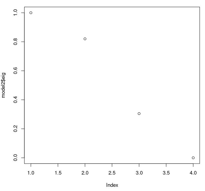
R reports the eigenvalues in order of magnitude. We see the first three are substantial, and the fourth is tiny. It is worth noting that the fourth is positive, so our distances are euclidean.
Plotting the 2D model, we get:
> plot(model2$points,asp=1,xlim=c(-0.8,0.8),ylim=c(-0.8,0.8))
> text(model2$points,labels=mylabels,pos=4)
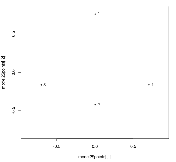
Warning: Note that it is critical to get the scaling the same in both dimensions. If we do not have this, then we cannot judge distances visually. The "asp=1" gives us a square plot, and the equal x- and y- ranges (specified by "xlim=c(-0.8,0.8),ylim=c(-0.8,0.8)" which say that -0.8 ≤ x ≤ 0.8 and -0.8 ≤ y ≤ 0.8) achieve this. (In R, the "c" specifies a list or vector of values.)
Let's compare distances in the model to our original distances.
    > as.matrix(dist(model2$points))
              1         2         3        4
    1 0.0000000 0.7537229 1.4142136 1.167820
    2 0.7537229 0.0000000 0.7537229 1.190367
    3 1.4142136 0.7537229 0.0000000 1.167820
    4 1.1678200 1.1903667 1.1678200 0.000000
    > D
             [,1]     [,2]     [,3]     [,4]
    [1,] 0.000000 1.000000 1.414214 1.224745
    [2,] 1.000000 0.000000 1.000000 1.224745
    [3,] 1.414214 1.000000 0.000000 1.224745
    [4,] 1.224745 1.224745 1.224745 0.000000
    >
Here we have the distances calculated with the points in the model, and then our original distances.
We can see that some values are exactly the same, but others are not. We can subtract to make an easy comparison:
    > D-as.matrix(dist(model2$points))
             1          2            3          4
1 0.000000e+00 0.24627705 2.220446e-16 0.05692492
2 2.462771e-01 0.00000000 2.462771e-01 0.03437813
3 2.220446e-16 0.24627705 0.000000e+00 0.05692492
4 5.692492e-02 0.03437813 5.692492e-02 0.00000000
> max(D-as.matrix(dist(model2$points)))
[1] 0.2462771
We see that the maximum deviation from the true distance is about 0.246,
which is substantial given the size of the original distances (all between 1 and 1.5).
In fact, we can divide by the entries in the original matrix:
> (D-as.matrix(dist(model2$points)))/D
             1          2            3          4
1          NaN 0.24627705 1.570092e-16 0.04647900
2 2.462771e-01        NaN 2.462771e-01 0.02806963
3 1.570092e-16 0.24627705          NaN 0.04647900
4 4.647900e-02 0.02806963 4.647900e-02        NaN
> max((D-as.matrix(dist(model2$points)))/D,na.rm=TRUE)
[1] 0.2462771
With this we can see that the maximum percentage error is about 24.6% (quite large, at least in some contexts) and this occurs for several of our distances.
MDS does not "try" to keep percentage error to a minimium: it opimizes for mean square error, and minimizes that. As a result, it is possible to get non-tiny percentage errors, even if the model is quite good. Generally, these large percentage errors will be associated to the smallest distances in the data.
Let's plot the distances of the model against the original distances:
> plot(as.dist(D),dist(model2$points),asp=1,xlim=c(0.7,1.4),ylim=c(0.7,1.4))
> abline(0,1)
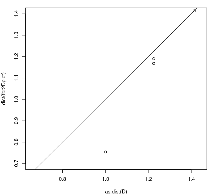
The first command plots the original distances as x-coordinates and the model distances as y-coordinates. Again, I have set the x- and y- ranges to be identical, with an aspect ratio of 1. The abline command adds the line y=x (0 intercept and slope 1) to the plot. This is key: we want to compare how the points in the scatter plot compare to the line y=x. We can see the large discrepancy between the point around (1.0,0.75) (note how far it is below the y=x line). This again shows that the model is not great.
Moving on to 3D, we create the 3D model like this:
> model3 <- cmdscale(D,k=3,eig=TRUE)
The points in the model are:
    > model3$points
                  [,1]       [,2]       [,3]
    [1,]  7.071068e-01 -0.1671134 -0.2565601
    [2,]  4.440892e-16 -0.4280699  0.4006322
    [3,] -7.071068e-01 -0.1671134 -0.2565601
    [4,] -8.326673e-17  0.7622968  0.1124881
Comparing distances, we find the model distances to be exactly the same as the input distances:
    > dist(model3$points)
             1        2        3
    2 1.000000
    3 1.414214 1.000000
    4 1.224745 1.224745 1.224745
    > as.dist(D)
             1        2        3
    2 1.000000
    3 1.414214 1.000000
    4 1.224745 1.224745 1.224745
    > dist(model3$points)-as.dist(D)
                  1             2             3
    2  2.220446e-16
    3 -2.220446e-16  4.440892e-16
    4  4.440892e-16 -2.220446e-16  4.440892e-16
The tiny differences are non-zero simply due to lack of infinite precision in computations.
Plotting the distances of the model against the original distances yields:
> plot(as.dist(D),dist(model3$points),asp=1,xlim=c(0.7,1.4),ylim=c(0.7,1.4))
> abline(0,1)
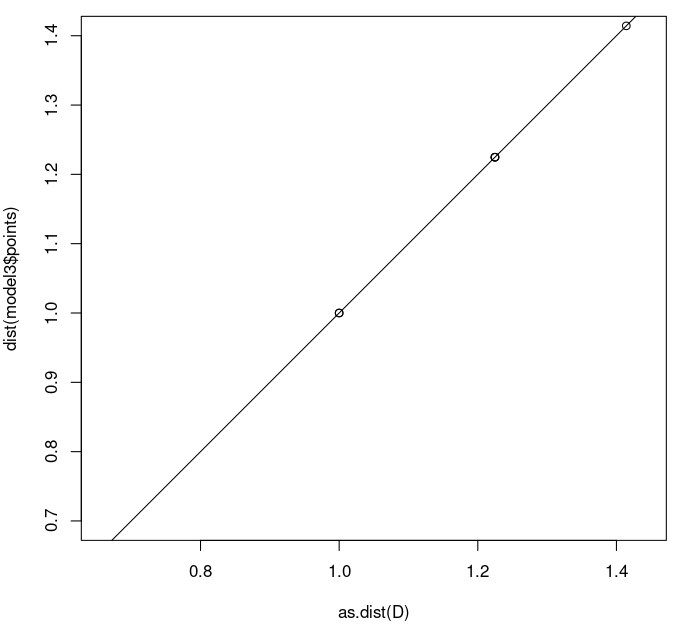
We see that all points are now right on the y=x line, since the model distance and the input distances are now the same.
So, MDS is able to get our points located in 3D space with the same relative positions as our original points.
With real world data that involves actual measurements or estimations of distances, we will never have quite so close a fit.