Plotting discrete fourier transforms for integer sequences

Suppose we have an increasing sequence of positive integers {a_n}. We can investigate some of the sequences spectral properties through the function f_N(x) = sum_i=1,N cos(a_nx). The function is periodic with period 2pi, so when plotting we need only consider 0 ≤ x ≤ 2 π.

For any sequence, we have f(0,N) = f(2pi,N) =N .

Note that, since a_n is an integer, then cos(a_nx)=cos(a_n(2pi-x)) for all sequences and all x. As a result, all plots of f_N(x) will be symmetric about x=pi.

If the sequence is essentially random, we can expect f_N(x) to be roughly the size of the square root of N. So by noting where the f_N(x) is large in magnitude can indicate a tendency to be distributed in certain ways with respect to certain frequencies.

For example, consider the sequence {a_n} = {5n}. Calculating f_N(x) for this sequence, we find that f_N(x) = 100 exactly when x is a multiple of 2pi/5, and otherwise it is much smaller.

This tells use that the waveform created by the seqence {5n} will have peaks at intervals of 2pi/(2pi/5 = 5, which is no big surprise, of course. However, working with any sequence, this method can be used to find strong spectral components of the waveform, by observing for what values of x f_N(x) is large.

Primes

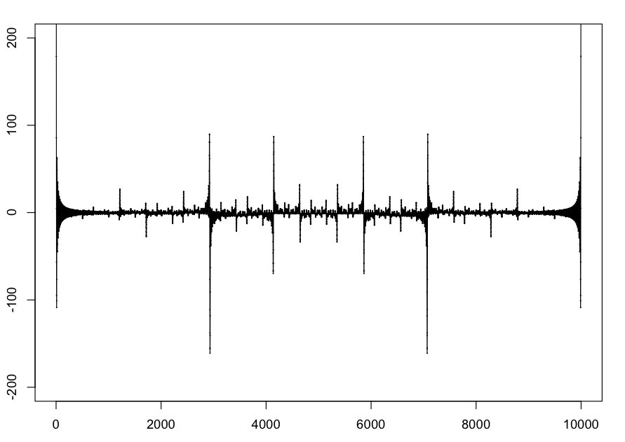
Let's look at f_N(x) for the sequence of primes. Let's use N=300. In GP, we can generate a list of the values of f(x,N) = sum(cos( prime_i x)) where i runs from 1 to N and prime_i is the i-th prime. In GP, execute the following commands:

f(x,N) = sum(i=1,N,cos(prime(i)*x))
for(j=0,10000,print(f(j*2*Pi/10000,300)))

Read the output into R and plot:

> primes1 <- scan("primes300-10000.txt")
> plot(primes1,xlim=c(0,10000),cex=0.1)
> lines((primes1))

The output x axes is labeled with the index of the point plotted. So the point with x coordinate m has actual x value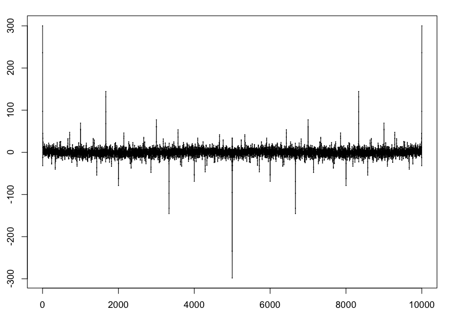
2pi m/10000. This yields the following plot:

Let's observe some features of this plot:

There is a major negative value at x=pi. Since cos(pi*prime(i))=-1 except for i=1, f(pi,N) = -N+1. Conversely, the large negative values of f(pi,N) indicates that the vast majority of primes are odd.
There is a large negative values at x=2pi/3. Since all primes except 3 are not divisible by 3, and cos(2pi/3 k) = -1/2 when k=1 or 2, we see that f(2Pi/3,N) = -N/2+1.
There is a large positive value at x=2pi/6. Since all primes greater than 3 are congruent to 1 or 5 mod 6, and cos(2pi/6*1)=cos(2pi/6*5)=0.5, we see that f(2pi/6,N) = N/2-3/2.
There is a noticeable negative spike at x=2pi/5. Since all primes greater than 5 are not divisible by 5, and the primes are uniformly distributed among the other residue classes mod 5 (see Prime Number Theorem for Primes in Arithmetic Progression), we can expect that f(2pi/5,N) to be approximately
N((1/5)(cos(2pi/5)+cos(4pi/5)+cos(6pi/5)+cos(8pi/5))) ≈ -N/5.

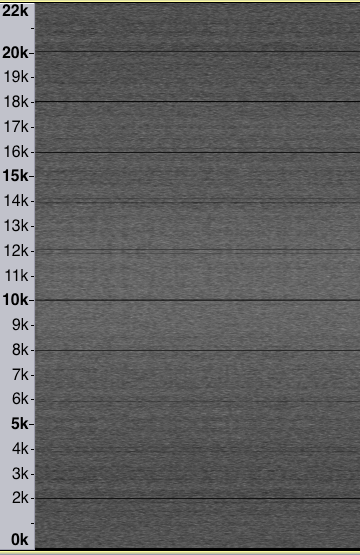
For the primes sequence, the prominent spikes in the plot of f(x,N) correspond to spectral lines in the spectrograms of the waveforms we make: if the spike is at x, then the frquency in the spectrogram is 44100x/(2pi). Note that we only plot the spectrograms up to the Nyquist frequency (half the sampling rate, 44100/2-22050).

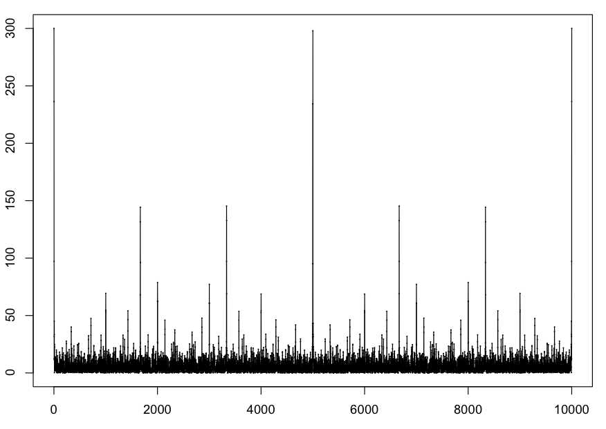
Also, the spectrogram and the "plot spectrum" functions in Audacity only consider the absolute values of the spectral components, so it be sometimes useful to use the R command

> plot(abs(primes1),xlim=c(0,10000),cex=0.1)
> lines(abs(primes1))

to get a more easily comparable figure. Here is the result for the command above:

Ulam numbers

The ulam sequence is defined here. Here is a plot of f(x,500) for this sequence, with 10000 points.

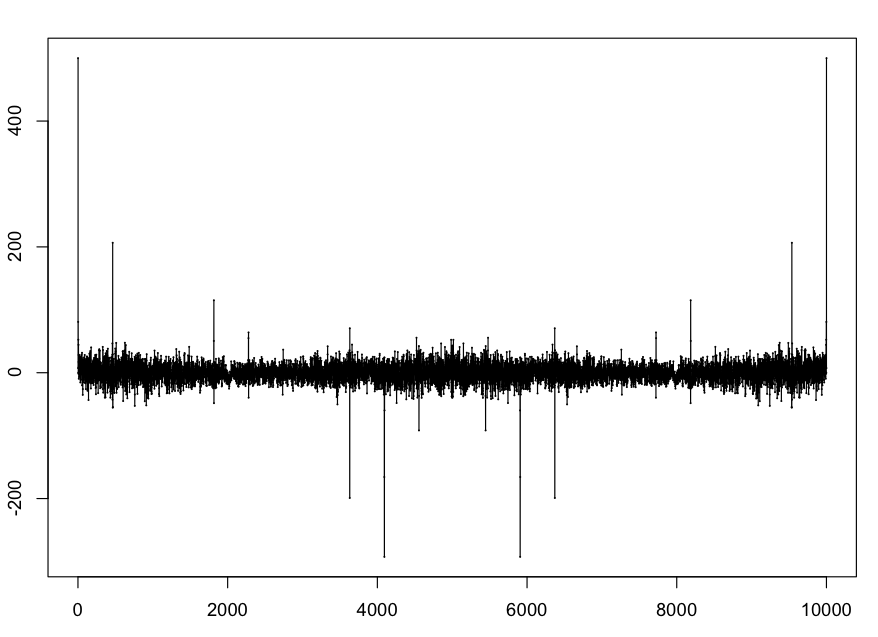
The spike at around 464 (i.e., 0.29154) corresponds to the line in the spectrograph of our waveform for this sequence at approximately 2046 hz. This also corresponds to the known "clumping" phenomenon of the sequence which has period 21.6 (44100/2046 is about 21.6).

The major negative spike around the 4000th point is at x=2.57... . Stefan Steinerberger has shown the surprising fact that there exists a value A=2.57... such that, with only four exceptions, for all Ulam numbers a_n up to (at least) 10⁷, cos(Aa_n)<0. This 2.57.. value corresponds to a spectral line around 18048 hz that is visible in the spectrogram for the soundfile:

Beatty sequence for the square root of 2

The Beatty sequence of the square root of 2 is the sequence a_n = floor( nb ) where b is the square root of 2.

Here is the plot with N=500 and 10000 points.

This one seems to have the possibly interesting feature of having large positive and negative spikes quite close together.